Single-mode fiber guides one fundamental spatial mode at its specified operating wavelength. “9/125” is a common nominal telecom geometry, not the fixed size of every single-mode fiber. High-power laser fibers require designs suited to wavelength, mode quality and power conditions.
This article answers one question: how to read single-mode fiber specs? The answer has four layers: the single-mode condition (V parameter), the G.652/655/654/657 standards, MFD and dispersion, and OS1/OS2 attenuation.
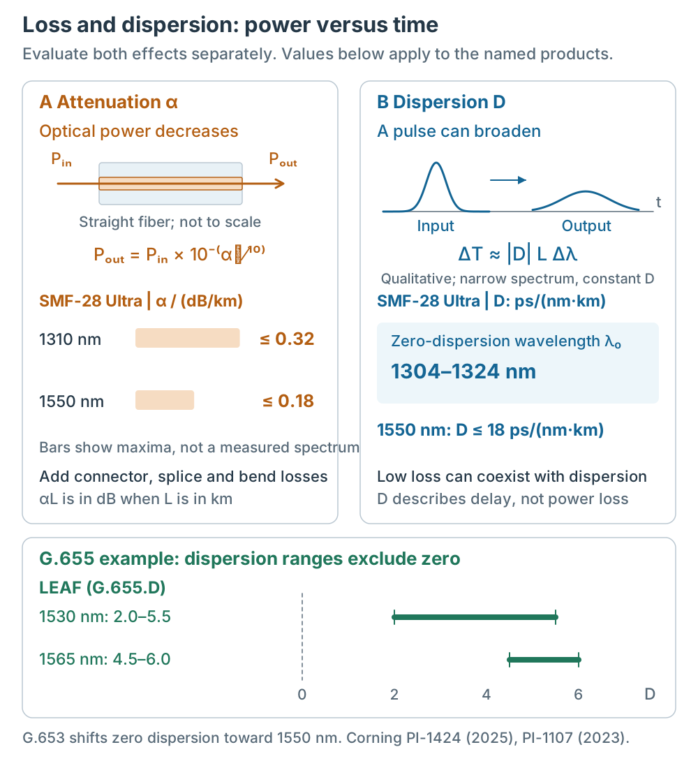
Figure 1 | The left column tracks power loss; the right tracks group delay and possible pulse spreading. Attenuation bars represent product maxima at specified wavelengths, not measured spectra. LEAF intervals stay clear of zero, distinguishing G.655 from G.653. Pulse shapes are qualitative; numbers follow the named product datasheets [5–8]. Click any figure for full size.
1. Single-Mode Condition: V Parameter, 9/125
For a weakly guiding step-index model, the single-mode condition is V < 2.405: V = 2π·a·NA/λ, with core radius a, index-derived numerical aperture NA and wavelength λ. At fixed NA, a smaller core or longer wavelength reduces V. Other index profiles require their corresponding model[9].
“9/125” specifies approximately 9 μm core / 125 μm cladding. Single-mode operation still depends on NA and wavelength. Figure 2 assumes a =4.5 μm and NA =0.12, giving V ≈2.59 at 1310 nm and ≈2.19 at 1550 nm. This is a step-index teaching example, not a G.652 product specification.
A 9 μm core needs micron-level alignment when coupling to a laser or detector, one reason single-mode costs more than multimode — a 50 μm multimode core couples loosely, while a 9 μm single-mode core needs precise alignment.
Single-mode has one mode, so there is no modal dispersion (different modes traveling at different speeds) — this is the root reason single-mode reaches far.
V is a normalized frequency that determines the model’s guided-mode conditions, not the mode count itself. Distinguish fiber and cable cutoff tests: SMF-28 Ultra specifies cable cutoff λcc ≤1260 nm, an upper limit rather than an identical exact cutoff for every fiber[5][9].
Check that the operating wavelength is within the product’s single-mode range, together with cutoff test conditions and the NA definition. A far-field power-threshold NA must not automatically be substituted into an ideal step-index equation.
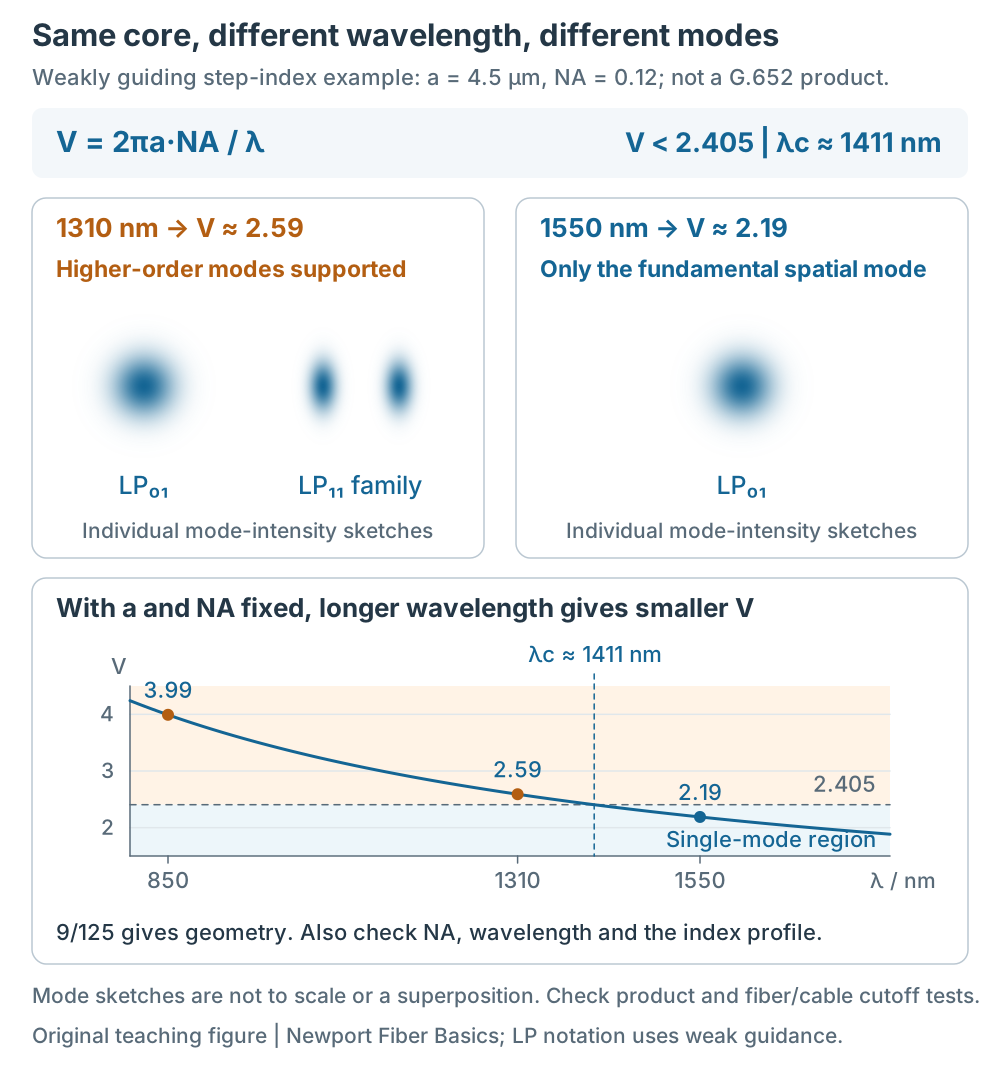
Figure 2 | This weakly guiding step-index example fixes a =4.5 μm and NA =0.12. It supports higher-order spatial modes at 1310 nm and only the fundamental at 1550 nm; λc ≈1411 nm is not a G.652 product cutoff. Spots illustrate individual mode-intensity shapes, not a superposition or computed eigenmodes. The lower curve shows V decreasing with wavelength at fixed geometry and NA [9].
Across Wavelengths and Products: Read MFD with the Model
Thorlabs offers single-mode fibers across ultraviolet, visible and near-infrared wavelengths. The following cross-band examples retain the product distinctions. Datasheet editions may differ; read MFD with its test wavelength, nominal value or range, and tolerance. Procurement and acceptance require the current datasheet for the specified model[12–14].
| Wavelength range | Product | MFD | NA |
|---|---|---|---|
| 320–430 nm | SM300 | 2.0–2.4 μm at 350 nm | 0.12–0.14 |
| 405–532 nm | SM400 | 2.5–3.4 μm at 480 nm | 0.12–0.14 |
| 488–633 nm | SM450 | 2.8–4.1 μm at 488 nm | 0.10–0.14 |
| 633–780 nm | SM600 | 3.6–5.3 μm at 633 nm | 0.10–0.14 |
| 780–970 nm | 780HP | 5.0 ±0.5 μm at 850 nm | 0.13 |
| 980–1550 nm | SM980-5.8-125 | 5.3–6.4 μm at 980 nm | 0.13–0.15 |
| 1260–1625 nm | SMF-28 family | 9.2 μm at 1310 nm; 10.4 μm at 1550 nm | 0.14 |
| 1850–2200 nm | SM1950 | 8.0 μm nominal at 1950 nm | 0.20 |
Within one fiber design, MFD changes with wavelength. SMF-28 Ultra specifies 9.2 ±0.4 μm at 1310 nm and 10.4 ±0.5 μm at 1550 nm[5]. But wavelength alone does not determine MFD across products: SM1950 has a nominal MFD of 8.0 μm at 1950 nm, smaller than that 1550 nm example[14]. Figure 3 compares these values on one scale.
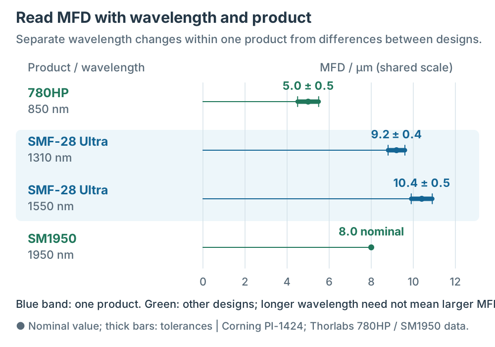
Figure 3 | The blue band contains one product at two wavelengths; green rows show other designs. Dots mark nominal values, thick bars the stated tolerances, and thin lines assist comparison against the common scale. SM1950 has only a nominal value here; no tolerance is invented. This is not a universal MFD curve connecting different products [5][13][14].
The a in the V equation is the physical core radius; do not directly substitute MFD/2. MFD describes the mode-field width, which can extend into the cladding. First confirm the product’s single-mode operating band, then check MFD, coupling and the other requirements.
2. G.652/655/654/657
ITU defines several single-mode fiber standards, each with a use[4]:
| Standard | Feature | Use |
|---|---|---|
| G.652 | standard SMF, zero-dispersion wavelength near 1310 nm | common telecom fiber |
| G.655 | NZDSF: dispersion magnitude remains non-zero in the specified band | some DWDM/long-haul systems |
| G.654 | cut-off shifted, low loss near 1550 nm; some types have larger effective area | submarine and long-haul transmission |
| G.657 | bend-insensitive | FTTH, tight bends |
- G.652: zero-dispersion wavelength near 1310 nm, often with lower attenuation at 1550 nm. Subclasses have different parameter and test requirements. Read the standard edition and product datasheet; the D label is not one fixed set of product values[5].
- G.655 (NZDSF): retains non-zero dispersion across 1530–1565 nm to reduce certain DWDM nonlinear effects. It must not be drawn as zero dispersion at 1550 nm; shifting the zero-dispersion region toward 1550 nm describes G.653[7][8]. The LEAF (G.655.D) example specifies 2.0–5.5 ps/(nm·km) at 1530 nm and 4.5–6.0 at 1565 nm, both non-zero[6].
- G.654: cut-off shifted and designed for low-loss transmission in the 1550 nm region. Some types use larger effective areas to reduce nonlinearity. Check subclass and operating-band compatibility[11].
- G.657: bend-insensitive, tolerates tight bends, for FTTH (fiber to the home).
Selecting a standard requires checking the system band, distance, dispersion tolerance, nonlinearity and compatibility with existing fiber. DWDM is not limited to G.655; systems also use G.652 or G.654. G.657 bend tolerance must be read with the model, wavelength and bend-test conditions, not taken as free to bend tightly.
3. MFD and Dispersion
MFD (mode field diameter) is the effective mode-field size, read with wavelength, definition and tolerance[1]. SMF-28 Ultra specifies 9.2 ±0.4 μm at 1310 nm and 10.4 ±0.5 μm at 1550 nm[5]; these are not fixed values for all G.652 fibers. Coupling depends on field overlap[10]. Under coaxial, same-polarization, same-wavelength Gaussian assumptions with coplanar waists, Figure 4 uses η = [2w₁w₂/(w₁²+w₂²)]² for pure MFD mismatch. The 10.4/12 μm example gives η ≈0.980 and approximately 0.089 dB loss. Actual splices also depend on offset, tilt, field shape and end-face conditions.
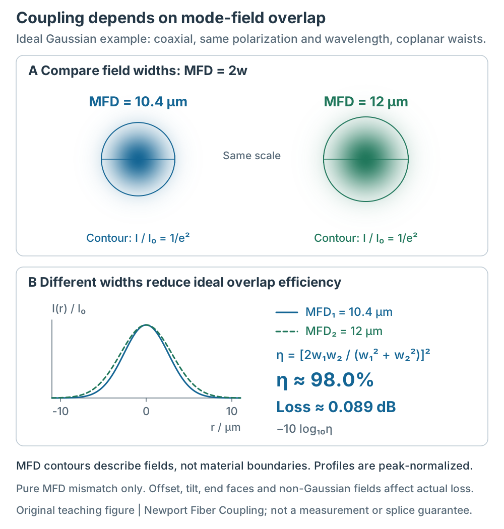
Figure 4 | Compare field widths, then overlap efficiency. Here MFD =2w uses the Gaussian definition: intensity at radius w is 1/e² of its peak. The contour is not a core boundary. Profiles are individually peak-normalized; η comes from normalized field overlap. No other interface loss is included, so the example does not predict actual splice performance [10].
Dispersion: G.652 has a zero-dispersion wavelength near, not necessarily exactly, 1310 nm. Figure 1 uses SMF-28 Ultra limits: λ₀ =1304–1324 nm and D ≤18 ps/(nm·km) at 1550 nm[5]. For the same product:
- 1310 nm: near the zero-dispersion region; maximum specified attenuation is 0.32 dB/km.
- 1550 nm: maximum specified attenuation is 0.18 dB/km; dispersion still requires checking.
The low-loss 1550 nm region supports long reach, but wavelength selection depends on transceiver, data rate, modulation and link budgets. It is not a universal low-speed/high-speed split. For a narrow spectrum and approximately constant D, ΔT ≈ |D|LΔλ estimates the dispersion delay spread[3]. Pulse chirp and compensation affect actual pulses; optical compensation or DSP depends on the system.
4. OS1/OS2 and Attenuation
OS1/OS2 are single-mode cabling categories. Common cabled-attenuation limit examples follow; check the applicable wavelength, test conditions and standard edition[2]:
- OS1: loss ≤ 1 dB/km (short reach)
- OS2: loss ≤ 0.4 dB/km (long reach)
OS2 is also common in short single-mode links; distance alone does not distinguish OS1 and OS2. The bare-fiber product limits in Figure 1 differ from cable and complete-link conditions. Add connector, splice and bend losses to a link budget. Check low-water-peak performance at 1383 nm rather than drawing a universal high OH peak[5].
5. Applicable Range and Limits
Single-mode fiber suits long-reach, high-speed, high-power applications. It reaches far (low loss, no modal dispersion) and is the backbone of long-haul communications.
Typical applications: long-haul communications, datacenter interconnect (DCI), high-power fiber lasers, sensing. A high-power fiber laser uses single-mode fiber for the signal light (9 μm core), maintaining beam quality (M² close to 1[15]); the pump light uses large-core fiber (20–100 μm[16]) — because the pump power is high, a large core lowers the power density (see the specialty fiber article).
Splicing requires a process compatible with the fiber type, with alignment, loss and mechanical strength verified. MFD matching reduces field-mismatch loss but does not replace measured splice acceptance.
Limits:
- small core (9 μm), coupling is hard and needs precise alignment
- splice/coupling cost is higher than multimode
- 1550 nm needs dispersion management
Read nominal geometry, operating wavelength/cutoff, ITU type, MFD, dispersion and cabled attenuation individually. Select for the system’s supported fiber and band, then check loss, dispersion, bends and coupling conditions.
The practical sequence: confirm the system and operating band, check the fiber and cable category, budget loss and dispersion, then confirm MFD, connectors and installation conditions. Write the specific model and test conditions into the spec sheet instead of treating typical values as guaranteed.
Common Misconceptions
- “Single-mode is always better than multimode”: Wrong. Single-mode reaches far but couples hard and costs more; multimode is cheaper and couples loosely, enough for short reach. Choose by distance.
- “All single-mode fibers are the same”: They are not. G.652/655/654/657 each have uses; OS1/OS2 loss differs too.
- “MFD is the core diameter”: MFD describes the field; core diameter is physical geometry. Read values with their design and wavelength conditions.
Self-Check for the Reader
- Can you state the single-mode condition (V parameter)?
- What is the difference between G.652 and G.655?
- Why does long-haul use 1550 nm rather than 1310 nm?
Back to the opening question: read single-mode conditions, ITU type, MFD, dispersion and cabled attenuation in sequence. Product limits and teaching calculations have different scopes and cannot be combined into a universal single-mode datasheet. The overview and specialty-fiber articles cover related parameters and uses.