Quantum Optics: When Does Light Need a Quantum Description?

Classical electromagnetism describes light as an electromagnetic wave, and that description holds in most situations. But when the light is weak enough that photons must be counted one by one, the wave description fails. The boundary between the two is not a property of the light itself; it is set by the measurement.

Quantum communication, quantum computation, and precision measurement all rely on the quantum nature of light. Knowing when the quantum description is needed — and when it is not — determines how these technologies are designed.

The answer has three criteria: when the photon number of the light must be resolved one by one (single-photon level), when the photon correlations are non-classical (g⁽²⁾(0) < 1), and when vacuum fluctuations affect the measurement. In those situations, light must be treated as a quantum field.

1. The Problem: Where the Classical Wave Description of Light Breaks Down

The problem began in 1900. To fit the blackbody radiation spectrum, Planck proposed that the energy of the radiating oscillators can only take discrete values E = nhν; this is the origin of the quantum concept^[1]. In 1905, Einstein extended this assumption to light itself: the energy of a single photon is E = hν, which explains the photoelectric effect^[2]. Classical wave theory predicts that the energy of photoelectrons should grow with light intensity; experiments show it grows with frequency, while intensity only sets the number of photoelectrons. In 1927, Dirac quantized the electromagnetic field and gave quantum optics its mathematical framework^[3]; the absorption and emission of photons became a quantum interaction between field and matter. In 1960, Maiman built the first laser^[4]. Before the laser, photon-correlation experiments could only use weak thermal light; the laser provided a stable single-frequency source and made it possible to attenuate light down to the single-photon level.

Most everyday light carries a large photon number: a 1 mW laser at a wavelength of 1550 nm emits about 7.8×10¹⁵ photons per second (computed from P/(hc/λ)). Such light is well described by the classical wave.

The direct experimental evidence appeared in 1977. Kimble and colleagues observed the resonance fluorescence of individual atoms: the photons arrive one by one, and the probability of two photons arriving simultaneously is lower than for any classical light — antibunching^[5]. A classical wave can produce bunching (photons arriving in clusters), but it cannot produce antibunching. This is the clearest dividing line between classical and quantum light.

2. The Principle: Quantization of the Electromagnetic Field and Quantum States of Light

Quantum optics treats each mode of the electromagnetic field as a quantum harmonic oscillator. A mode of frequency ω has energy H = ℏω(a^†a + 1/2), where a^† is the creation operator: each application adds one photon to that mode^[3]. The ground state is the vacuum, but the vacuum is not “nothing” — it has vacuum fluctuations. Vacuum fluctuations are not a small correction: they set the noise floor of any measurement.

Light can be in different quantum states. The Fock state |n⟩ contains exactly n photons; the photon number is definite while the phase is completely undefined — a definite photon number comes at the price of a completely undefined phase. The coherent state |α⟩ is the ideal output of a laser: its photon number follows a Poisson distribution, and it is the quantum state closest to a classical wave^[6]. A squeezed state pushes the fluctuations of one quadrature below the vacuum level, at the price of increased fluctuations in the other quadrature — the uncertainty relation does not allow both to shrink at once. In 2007, Ourjoumtsev and colleagues generated an optical cat state — a superposition of two coherent states — directly from a photon number state^[7].

With the quantum description you can compute the full photon-number distribution and correlation functions of all orders; the classical description gives only the mean field and the intensity. The difference between the two shows up exactly in single-photon-level measurements.

3. The Principle: The Criterion for Non-Classical Light, g⁽²⁾(0)

Glauber gave light a quantitative criterion for “how quantum it is”: the normalized second-order correlation function g⁽²⁾(0) = ⟨n(n−1)⟩/⟨n⟩²^[6]. Substituting the photon-number distributions of the three standard states into the definition gives:

• Coherent light: g⁽²⁾(0) = 1 (Poisson distribution)
• Thermal light: g⁽²⁾(0) = 2 (bunching)
• Ideal single-photon source: g⁽²⁾(0) = 0 (antibunching) — no classical light reaches this

The correlation function of classical light is positive-definite, so any classical light has g⁽²⁾(0) ≥ 1; measuring g⁽²⁾(0) < 1 is evidence of non-classical light.

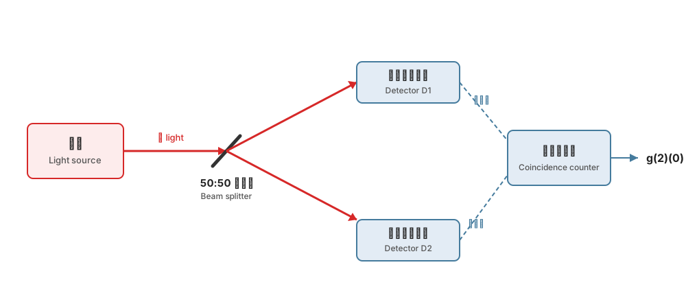
The measurement uses a Hanbury Brown–Twiss (HBT) setup: a 50:50 beam splitter divides the light into two paths, two single-photon detectors record the arrival times, and a coincidence counter computes g⁽²⁾(0) from the time correlation (see figure). The coincidence counter records how often the two detectors click within a time difference τ; g⁽²⁾(0) is the normalized coincidence rate at τ = 0. In 1977, Kimble and colleagues used this method to observe antibunching in the resonance fluorescence of a single atom^[5]. In 1986, Grangier and colleagues sent single photons into a beam splitter and observed that the two output ports never click simultaneously — a photon is indivisible^[8].

4. The Limits: The Applicable Boundary of the Quantum Description

The quantum description is not always necessary. When the mean photon number ⟨n⟩ is large, the relative photon-number fluctuation 1/√⟨n⟩ is small, and the classical wave description is sufficient. Radio communication, fiber-optic communication, and most laser-processing applications all use the classical description. The criterion depends on the measurement, not only on the source: the same laser light, once attenuated to the single-photon level, needs a quantum description.

Quantum optics itself has boundaries. It presupposes the framework of quantum mechanics and does not resolve the measurement problem: it describes how light and matter interact, not why a measurement yields the result it yields.

Common Misconceptions

1. Photon = tiny ball. A photon is an excitation of a field mode, not a classical particle. It has no definite trajectory, and its “position” is defined only by the measurement setup.
2. Vacuum = nothing. The vacuum has vacuum fluctuations. In 2011, Wilson and colleagues rapidly modulated the boundary of a microwave cavity with a superconducting circuit (equivalent to a mirror moving at a significant fraction of the speed of light) and generated real photons from the vacuum — the dynamical Casimir effect^[9].
3. Laser light is “already classical enough.” Coherent light is the most classical of quantum states, but it still has Poisson photon-number fluctuations (shot noise). Shot noise sets the limit of weak-light measurements: coherent light with N photons has a relative photon-number fluctuation of 1/√N.

5. The Answer: When Light Needs to Be Described by Quantum Mechanics

Back to the opening question. Light needs a quantum-mechanical description in three situations. First, when the photon number must be resolved one by one (single-photon level). Second, when the photon correlations are non-classical (g⁽²⁾(0) < 1). Third, when vacuum fluctuations affect the measurement (squeezed light, radiation-pressure noise).

These criteria are not just theoretical. The KLM scheme proposed in 2001 showed that linear optical elements plus photon detection can implement universal quantum computation^[10]. Quantum key distribution uses single photons to carry keys; the Micius satellite distributed entangled photons over 1200 km in 2017^[11]. LIGO injects squeezed vacuum states to suppress quantum noise^[12]. Haroche’s cavity QED experiments measured and manipulated individual photons, earning the 2012 Nobel Prize in Physics^[13].

The practical check is direct: build an HBT setup and measure g⁽²⁾(0); a value below 1 means the light is non-classical. What the sources have not yet resolved: there is no fundamental dividing line between classical and quantum; the boundary is set by the noise floor of the measurement, and the measurement problem itself lies outside the scope of quantum optics.

Self-Check Questions for the Reader

1. Why can a classical wave produce bunching but not antibunching?
2. What is the value of g⁽²⁾(0) for laser output? What does this value mean?
3. What is the difference between the vacuum and “nothing”? Name one experimental evidence.