The quality of a high-speed digital signal cannot be judged from a single symbol’s waveform. One bit may look clean, but across a whole data stream, each symbol’s amplitude, arrival time, and rise shape differ slightly. These differences come from channel loss, reflections, clock jitter, and noise, and they accumulate to determine whether the receiver decodes correctly. The question is: how do you see the quality of an entire stream in one picture?
The eye diagram is the answer. It overlays all the symbols of the signal, making the statistical degradation—jitter, inter-symbol interference, noise—visible. A wide-open eye means good signal quality; a closed eye means there is a problem.
An eye diagram shows how many acquired samples occupy each amplitude and clock-relative phase. The unit interval (UI) is a symbol period: 1 UI = Ts = 1/Rs. It is a bit period for NRZ, whereas one PAM4 UI carries 2 bits. Eye height and width describe amplitude and timing margin under stated measurement rules; finite eye data alone cannot establish BER[3][6].
1. Why a Single Waveform Is Not Enough
A single symbol’s waveform only reflects the shape of “this one bit.” But bit errors in high-speed communication come from the statistical behavior of the whole stream: one symbol’s amplitude is a bit low, one transition arrives a bit early, one bit is polluted by residual energy from the previous bit. These effects are invisible in a single waveform, yet they accumulate into errors.
The eye diagram compresses this statistical behavior into one picture. It does not measure “one symbol”; it measures “the result of all symbols overlaid.” That is why high-speed signal quality assessment uses an eye diagram rather than a single waveform.
2. How an Eye Diagram Is Formed: Overlaying All Symbols
To form an eye, align waveform windows to a common symbol-clock or recovered-clock reference and overlay them. A two-UI display shows two symbol intervals; the construction in Figure 1 uses four consecutive two-UI windows. Aligning every data edge to itself would hide its relative timing variation. The displayed jitter also depends on the clock-reference method[3].
The horizontal axis is clock-relative time; the vertical axis is amplitude. Color-graded displays commonly count hits in amplitude/time bins. Brightness therefore shows sample occupancy, not an automatically calibrated probability density. A PDF interpretation additionally requires specified bins, conditioning and normalization[3].
Why does it look like an eye? A digital signal switches between the “1” and “0” levels. Overlaid, the “1” level forms a band on top, the “0” level a band on the bottom, the switching transitions form diagonal lines on the sides, and an eye-shaped opening remains in the middle. The better the signal quality, the more open the eye; the worse the quality, the more closed the eye.
The technique was first used with the WWII SIGSALY secure speech transmission system[1].
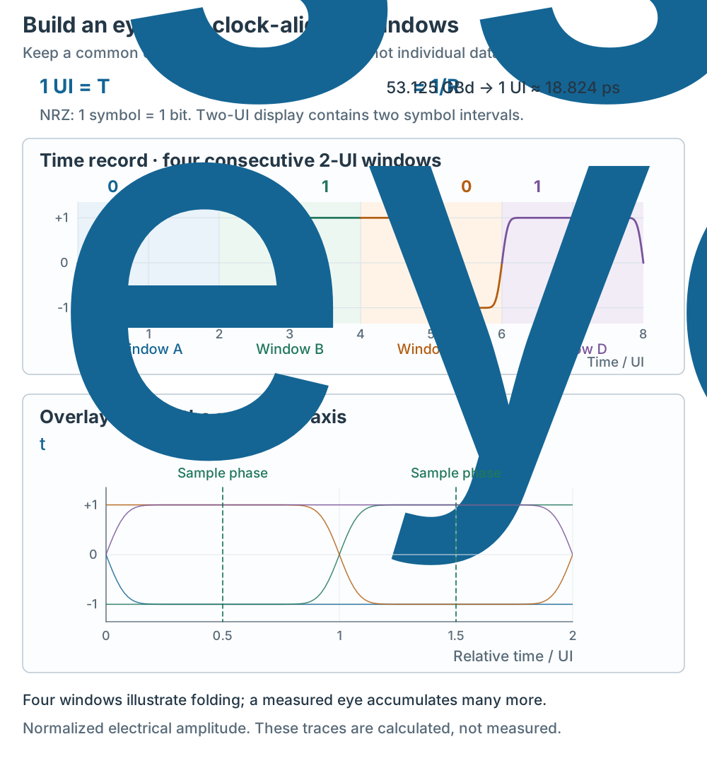
Figure 1 | The same waveform samples move from a time record to a relative-time eye. Four windows illustrate the construction. The dashed phases at 0.5 and 1.5 UI are sampling examples, separate from the crossings at 0, 1 and 2 UI. Normalized electrical amplitudes; calculated traces.
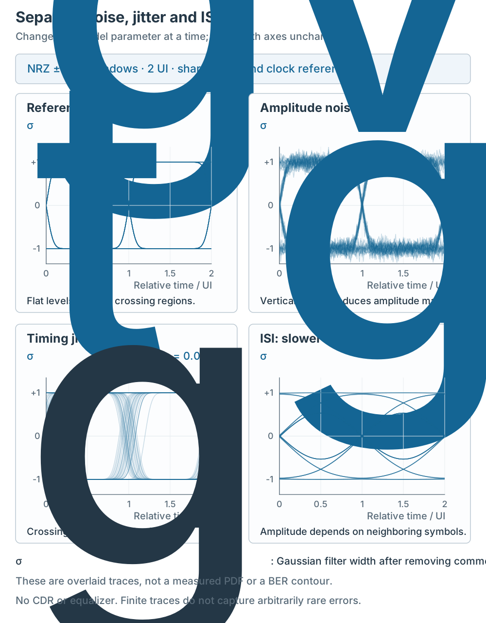
Figure 2 | Each panel changes one parameter, with the same scales and 72 two-UI windows. Gaussian low-pass response width σg models pulse spreading after removal of common delay. Gaussian noise or boundary jitter is added separately. No CDR or equalizer is modeled; trace overlap is not a measured PDF or BER contour.
3. How to Read an Eye Diagram: What Each Parameter Means
The eye opening comes in height and width, each corresponding to a kind of margin. The table lists the main features, what each represents, and what degrades it:
| Eye feature | What it represents | What degrades it |
|---|---|---|
| Eye height | Vertical opening at a specified sample window and statistical rule[4] | Amplitude noise, channel loss, poor extinction ratio |
| Eye width | Horizontal opening at a stated threshold and crossing-time rule[5] | Jitter |
| Transition width | Rise / fall time | Insufficient channel bandwidth |
| Distorted eye shape | Inter-symbol interference (ISI) | Channel reflections, dispersion |
| Blurred level bands | Amplitude noise | Thermal noise, relative intensity noise (RIN) |
Eye amplitude (the difference between level means) and eye height are distinct. For example, an SD algorithm subtracts 3σ from each level into the opening; eye width can likewise use inner 3σ boundaries of crossing-time distributions. Data-based and BER-target methods use other rules. State the algorithm, sample window and threshold before comparing numbers[4][5][8].
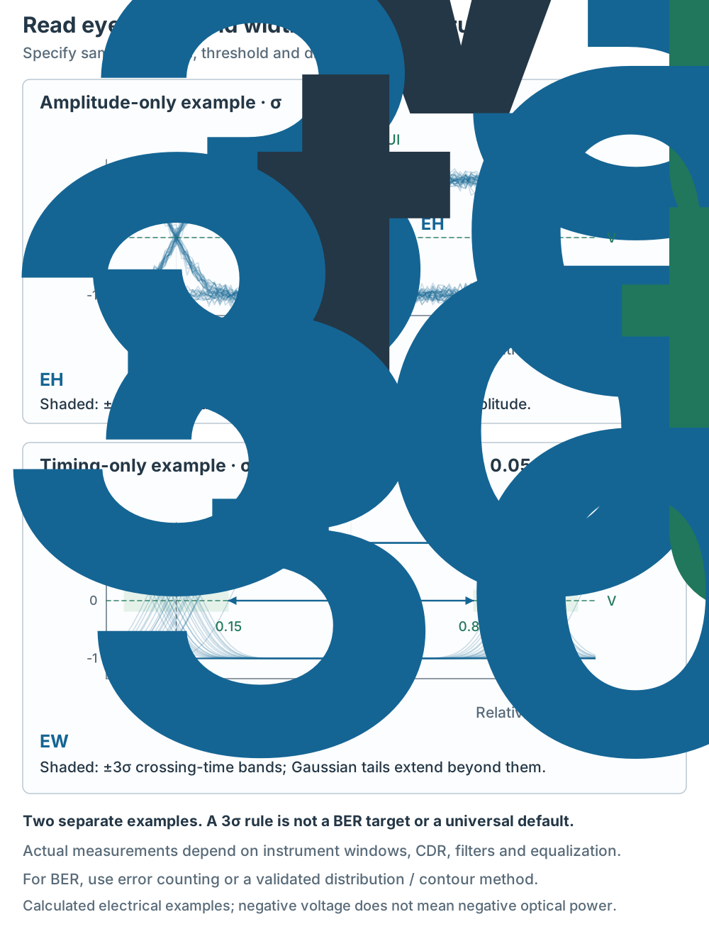
Figure 3 | A stated 3σ model gives EH3σ = 1.52 in normalized amplitude and EW3σ = 0.70 UI. The upper and lower panels are separate examples. Shaded bands are distribution boundaries, not measured extrema. A 3σ rule is neither a universal instrument default nor a BER claim.
Jitter is the timing variation of the transitions, in two classes[1]: random jitter (RJ) is commonly modeled as Gaussian and unbounded, with random sources such as thermal noise; deterministic jitter (DJ) is bounded, from signal-related sources such as ISI, crosstalk, and power-supply noise. Total jitter (TJ) is specified at a target BER, e.g. 10⁻¹². Jitter widens and blurs the transitions on both sides of the eye, directly eating into the eye width.
Inter-symbol interference (ISI) makes a symbol depend on neighboring symbols through the channel response. Figure 2 shows this using a slower low-pass model. Reflection severity depends on amplitude, delay and receiver processing; a delay longer than one UI alone does not prove that the eye is unreadable.
Extinction ratio (ER) is a parameter of optical transmitters, defined as the ratio of the average optical power of the “1” to the “0”: ER = 10 log10(P1/P0), in dB. Directly modulated transmitters are typically 6–10 dB, externally modulated systems can reach >20 dB; a poor extinction ratio shrinks the eye opening and raises the BER[2].
Other parameters include crossing percentage—the crossing amplitude relative to the logic-one and logic-zero means—and overshoot/undershoot. A symmetric electrical NRZ example crosses at roughly 50% amplitude, while its horizontal position depends on the chosen time origin. Figure 1 separates crossings from sampling phases[7].
An optical transmitter’s eye diagram shows how clearly the “1” and “0” optical power levels can be distinguished over time. The eye can be measured directly after the transmitter, or after a length of fiber; the latter’s degradation depends on the transmitter’s characteristics, in particular the chirp of a directly modulated laser[2].
4. What the Eye Diagram Cannot Show: Eye Closure vs BER
The biggest limitation of the eye diagram is: eye closure does not directly equal bit error rate. A partially closed eye does not let you read off a number like “BER = 10⁻¹².”
Why: the eye diagram shows the statistical distribution of the signal, but BER is the probability that the receiver actually decides wrong. To get a BER number, there are two paths:
- Bit error test: send a known pattern (e.g. a pseudo-random binary sequence, PRBS) and count the wrong bits over a period. Measuring a BER of 10⁻¹² requires measuring at least 10¹² bits (to expect one error); the lower the BER, the more bits are needed.
- Statistical model: fit the jitter and noise distributions (e.g. the dual-Dirac model) and integrate the distribution tails to estimate BER. Faster than a bit error test, but it depends on the model’s accuracy.
So the eye diagram is a “quick visual assessment” tool: it tells you whether the signal quality is good and where the problem comes from (jitter, ISI, noise), but getting a specific BER number requires an extra test or model.
Also, the eye diagram is a snapshot under specific measurement conditions. The trigger method, measurement point, and data pattern all affect the eye’s shape. When comparing two eye diagrams, the measurement conditions must match, or the difference may come from the measurement setup rather than the signal itself.
5. Answer
Back to the opening question: what is an eye diagram, why measure it, and what do the signals inside mean?
An eye diagram is a statistical plot of all symbols overlaid, showing the acquired distribution of amplitude versus UI phase. We measure it because a single waveform cannot show the accumulated statistical degradation. Eye height is amplitude margin, eye width is timing margin; jitter widens the transitions, ISI distorts the shape, noise blurs the level bands, and a poor extinction ratio shrinks the opening. But eye closure does not directly equal BER—getting a BER number requires a bit error test or a statistical model.
Common misconceptions:
- “Closed eye = high BER”: a finite eye can miss rare errors; neither visible closure nor an open eye by itself establishes a BER value[6].
- “The more open the eye, the better, at no cost”: an open eye requires sufficient bandwidth and SNR; PAM4 carries 2 bits/symbol and has three vertical openings between four levels. At equal peak amplitude, the vertical spacing is smaller; the horizontal eye width still depends on timing and channel conditions.
- “The eye diagram shows all problems”: it cannot show a BER number, nor certain degradations tied to specific data patterns.
Self-check:
- Why does the “eye” close? Name three factors.
- What margin does eye height correspond to, and what does eye width?
- Why can’t you read BER directly from eye closure? What do you need to get BER?