“Why does a 100G optical lane run at only 53.125 GBd? Can a 32 GHz device carry 100 Gbit/s?” These questions require three separate quantities: bits per second, symbols per second, and the width of the occupied frequency band.
The line rate comes from symbol rate and bits per symbol. Required bandwidth depends on pulse shape; reliable information transfer also depends on noise. The simplified models below establish the relationships before we apply them to link specifications.
Bit rate and symbol rate: separate the units
Bit rate is measured in bit/s, symbol rate in baud, and bandwidth in Hz. GHz describes a frequency interval, not a number of bits transmitted each second.
For M-level modulation with a fixed mapping of log2M bits per symbol, the raw line rate is:
Rline = Rs log2M
Rs is the symbol rate. Here M is a power of two and each symbol has a fixed bit mapping. Two-level NRZ (non-return-to-zero) carries 1 bit per symbol; PAM4 (four-level pulse-amplitude modulation) carries 2.
| Modulation | Bits per symbol | Symbol rate for the same 64 Gbit/s raw line rate |
|---|---|---|
| NRZ | 1 | 64 GBd |
| PAM4 | 2 | 32 GBd |
PAM4 therefore halves the symbol rate at the same raw line rate. Coding, forward error correction (FEC), and protocol overhead reduce the net useful rate Rnet. Raw line rate, nominal Ethernet rate, and application throughput need separate comparisons.
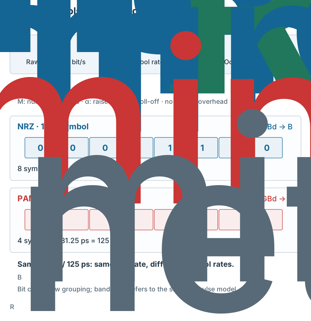
Figure 1 | Both formats transmit 8 bits in 125 ps: eight NRZ symbols or four PAM4 symbols. The cells show bit grouping. Bandwidth is calculated using a separate ideal pulse model; the cells are not rectangular band-limited waveforms.
Bandwidth limits: ideal pulses and real devices
Define a real, scalar baseband signal with spectrum from −B to +B; B is its one-sided occupied bandwidth. Ideal Nyquist pulses require at least Bmin = Rs/2 for zero intersymbol interference (ISI) at the sampling instants. This pulse-shaping condition does not make twice any device bandwidth a usable baud rate.[1]
For raised-cosine pulses with roll-off factor α between 0 and 1:
BRC = (1 + α)Rs/2
Zero roll-off gives the ideal minimum. At α = 0.25, 64 GBd NRZ occupies 40 GHz, while 32 GBd PAM4 occupies 20 GHz. Finite filters, the combined transmit/receive response, equalization, and the channel affect residual ISI.[1][2]
A device’s −3 dB bandwidth instead marks where response power falls to half its low-frequency reference. Frequencies above that point do not vanish abruptly. Optical spectral width, expressed in nm or THz, is another quantity. Driver, TIA, fiber, and complete-link bandwidth specifications are not interchangeable.[3]
Noise limits: PAM4 levels and Shannon capacity
PAM4 saves bandwidth but reduces level separation
Use DC-removed electrical amplitudes: NRZ levels are ±A; equally spaced PAM4 levels are −A, −A/3, +A/3, and +A. At the same peak, nearest-level spacing dmin falls from 2A to 2A/3. With the same Gaussian noise standard deviation σ, the distance to an ideal decision threshold also falls by a factor of three. Negative electrical amplitude does not mean negative optical power, and level spacing is not measured eye height.[1]
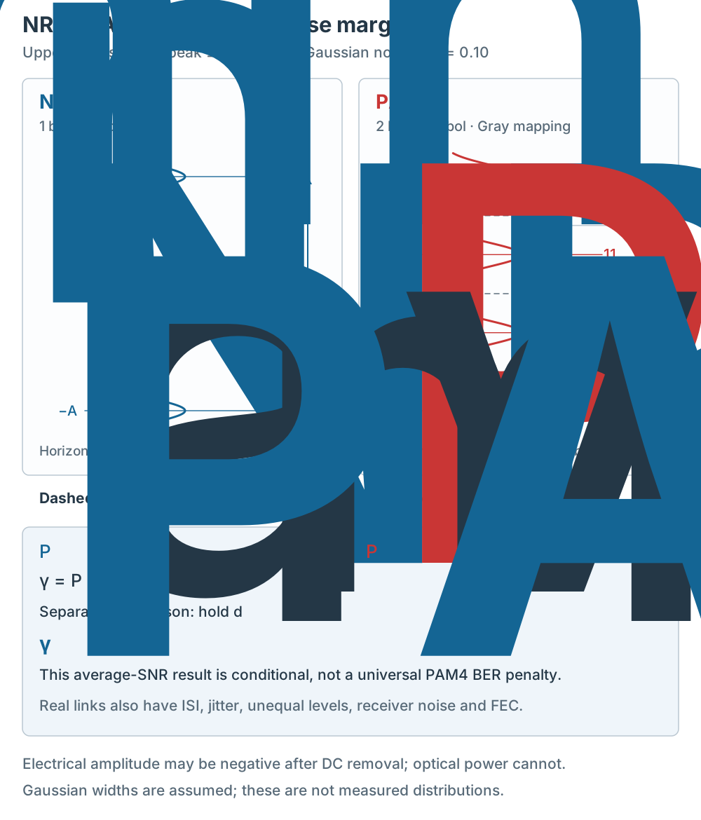
Figure 2 | The upper panels hold peak amplitude and σ/A = 0.10 constant. Horizontal width indicates per-level conditional probability density, not an eye diagram. The 6.99 dB calculation uses a separate comparison: fixed normalized threshold margin dmin/(2σ), allowing noise to change.
The “about 7 dB” statement needs a normalization. For equally likely levels and normalized mean-square electrical power, NRZ has Pavg = A2; PAM4 has 5A2/9. Holding dmin/(2σ) constant gives an average-power SNR ratio of 5, where γ = Pavg/σ2. Thus 10 log105 ≈ 6.99 dB. This model calculation is not a universal PAM4 BER or optical receiver-sensitivity penalty. Bit mapping, unequal levels, ISI, jitter, the receiver, and FEC change practical results.[1]
Shannon bounds information rate
For an ideal bandwidth-limited, average-power-limited additive white Gaussian noise (AWGN) channel, the Shannon–Hartley formula is:
C = B log2(1 + γ), with γ = 10SNRdB/10
C is information capacity in bit/s. γ is the received in-band signal-to-noise power ratio, entered as a linear value. An SNR of 20 dB means γ = 100; with B = 5 GHz, C ≈ 33.3 Gbit/s.[4]
For information rate Rinfo below C, coding exists in the ideal model that can make error probability arbitrarily small as block length grows. This does not guarantee zero errors in a finite practical system. Nor does C directly cap the number of raw coded bits sent per second: redundant bits do not all carry independent information. FEC improves reliability without increasing the capacity of the specified channel.[4]
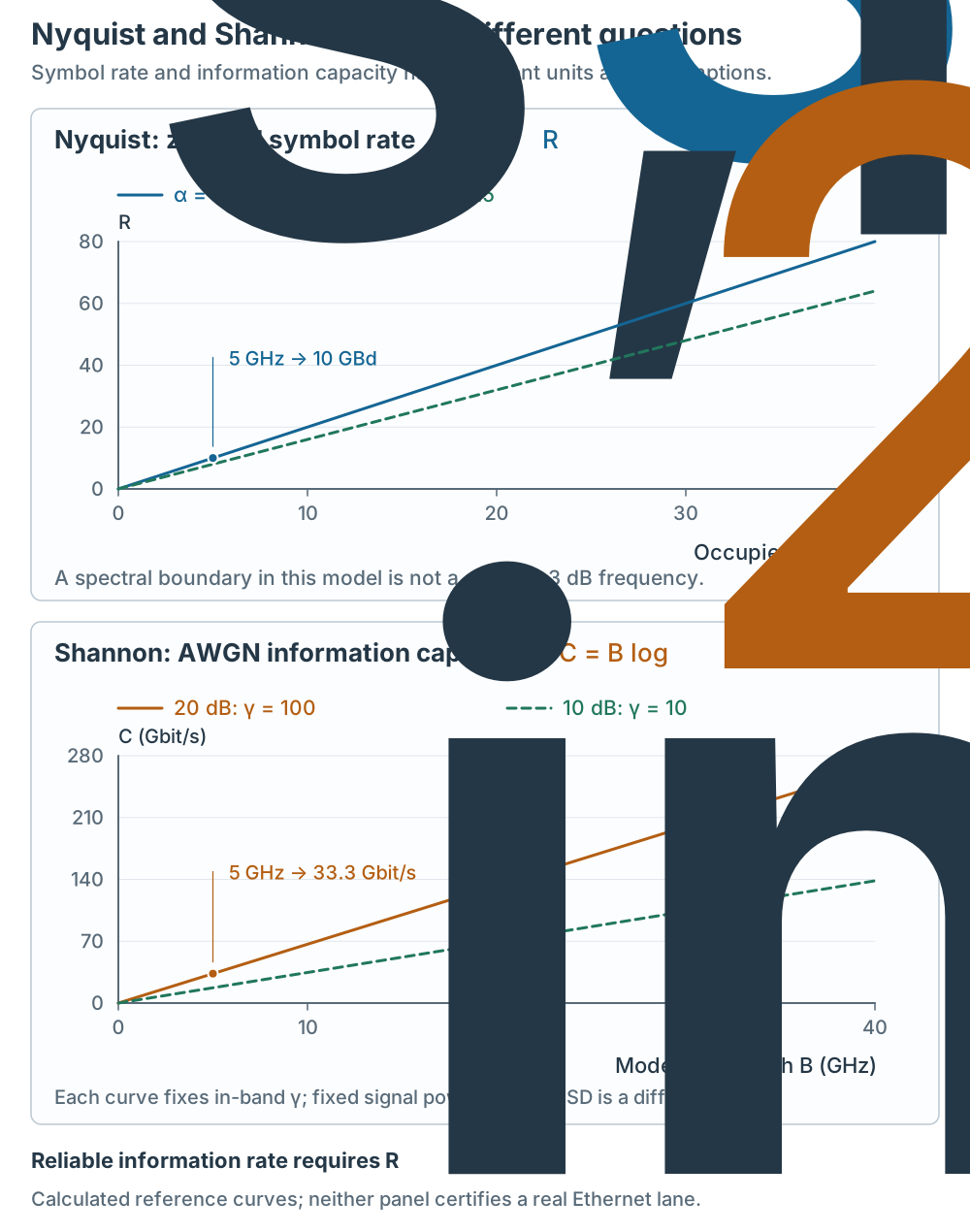
Figure 3 | The upper plot gives symbol rate in GBd for the pulse model; the lower gives ideal AWGN information capacity in Gbit/s. Each lower curve fixes in-band γ. With fixed signal power and noise power spectral density instead, γ changes with B, so these straight lines would not apply. Both plots are calculated examples.
Optical specifications: nominal rate, line rate and lanes
A 100GBASE-DR optical lane uses PAM4 at 53.125 GBd, corresponding to 106.25 Gbit/s of raw line rate. The difference from nominal 100G involves coding and FEC overhead. A raw 106.25 Gbit/s does not imply the same application throughput.[5]
| Explicit interface example | Modulation | Symbol rate per lane | Raw line rate per lane |
|---|---|---|---|
| 100GBASE-DR optical lane | PAM4 | 53.125 GBd | 106.25 Gbit/s |
| 200GAUI-1 electrical lane (P802.3dj public design example) | PAM4 | 106.25 GBd | 212.5 Gbit/s |
The second row is public IEEE task-force design material, not a claim about a final standard. Electrical AUI and optical lane counts can differ. That material describes 800GAUI-4 and 1.6TAUI-8 using nominal 200G per lane. “800G” alone does not imply eight 100G lanes; confirm the interface, modulation, and lane/wavelength configuration.[6]
In the pulse model above, 53.125 GBd with α = 0 gives Bmin = 26.5625 GHz. This is a pulse-model reference, not a guarantee that a TIA with 26.56 GHz −3 dB bandwidth meets a 100G link specification.
How to assess a real link
First align the rate level and test conditions, then evaluate bandwidth and reliability:
| Question | Specifications to check |
|---|---|
| Which rate is quoted? | Nominal interface rate, raw line rate, per-lane/per-wavelength rate, net throughput |
| How is bandwidth defined? | Device −3 dB, occupied pulse bandwidth, optical spectral width, fiber OFL/EMB |
| Can the receiver distinguish symbols? | Channel response, ISI, equalization, jitter, levels, noise |
| At what distance is operation reliable? | The specified PHY’s medium, loss, dispersion, launch conditions, BER and FEC criteria |
For example, OM4 has a minimum effective modal bandwidth (EMB) of 4700 MHz·km at 850 nm. Overfilled launch (OFL) is a different test condition.[7] Dividing 4700 MHz·km by 0.1 km gives 47 GHz only as a rough bandwidth-length-product estimate. Comparing it with 26.56 GHz does not establish a 100 m reach for a particular 100G PHY. Transmitter, receiver, launch conditions, loss, and error requirements also matter.
Single-mode fiber cannot simply be treated as having unlimited usable bandwidth: dispersion, sources, components, and noise constrain the link. Copper likewise requires frequency-dependent loss and equalization checks. Rate-to-bandwidth calculations provide a starting point; complete-link specifications and tests determine compliance.